Steps of efficiency determination

In order to determine the full-energy efficiency curve of a measurement system, first take some measurements with calibration sources (possibly with absolutely calibrated ones), and import them into your HyperLab database.

Our example will work with HyperLab's sample spectra belonging to a measurement setup with 70 keV – 3300 keV range. Please load the spectrum files into the database and also set their corresponding source values, as specified in section “Importing sample spectra”.

Perform a batch or individual evaluation on all measurements, and open a multi-line spectrum with the Peak evaluator. Check the FWHM and energy calibration, and adjust the region fits, if necessary. Finally save the peak list, which will be input for the efficiency evaluation.

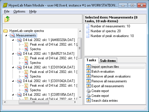
When all measurements are properly fitted, similar statistics will be displayed about them at the right side of the Main Module window as you can see in this picture.

To ease the work of the spectroscopist, the same peak evaluations may be utilized for nonlinearity determination and for efficiency analysis.

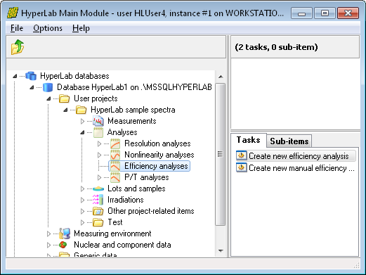
Open Analyses node under your project, then click on Efficiency analyses and select Create new efficiency analysis task.

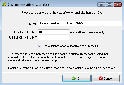
A new window appears now, where basic parameters of efficiency fitting algorithm may be specified.

Here you can specify a descriptive name of the new efficiency analysis, and thresholds for the identification of peaks.

The Peak identification limit is used when peaklist peaks and nuclear library peaks are matched.

If the difference between peak centroid and radiation's energy is below this Chi value (using the combined energy uncertainty value of the peak and gamma line), the peaks will be considered as matching.

Its usual value is 100 Chi, which is appropriate even for cases when nonlinearity correction is not applied in the energy calibration, therefore huge differences may occur for peak positions. If you are using nonlinearity correction for all of your measurements used for the efficiency analysis, enter a value of 5.0 Chi here.

The Radiation intensity limit is used when radiations are loaded for a selected decay from the database. The 0.005 default value load the radiations where the intensity is greater than 0.5% of the decay's strongest line. When you are ready, press OK.

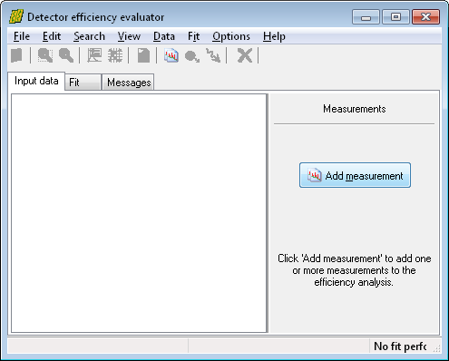
The Detector efficiency evaluator window appears now with the empty Input data sheet.

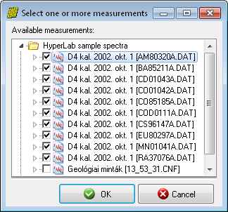
Click Add measurement button at the right. The Measurement selector window appears now.

Select all of HyperLab's example measurements from the project.

When you click OK in the measurement selector window, HyperLab performs the steps as follows.

Loads the peaks from the most recent peak evaluation of the measurement (this should be the nonlinearity corrected peaklist).
Checks if a radioactive source is specified for the measurement. If found, loads its isomers and their radiations, as well as source activity details. Otherwise prompts the user for selecting the isotopes.
Limits the radiations to those whose intensity is over the preset intensity limit and which have a radiation usage flag, enabling the radiation for detector efficiency evaluation purposes.
Matches the loaded radiations and their closest fitted peaks, by applying the preset matching limit.
If at least one matching peak-radiation pair is found within a peak list (or 2 matching pairs for measurements taken with a home-made source), then the measurement may be used for efficiency evaluation.
Checks if enough input data points exist for a polynomial fit. The number of data points must exceed the number of fitted parameters, i.e. the degree of the fitting polynomial plus one activity shifting parameter for each non-absolutely calibrated measurement.

If enough data points are identified, the fit will succeed and the tab Fit becomes active, displaying the fitted efficiency curve.

It will be an absolute efficiency curve if any of the matching measurements has an absolutely calibrated source, and it will be relative efficiency if no measurement has such source.

Now you can add other measurements to the fit one-by-one, or more at a time. Eventually, a multi-measurement, multi-isotope efficiency curve may be easily constructed.

Improvement of the fit

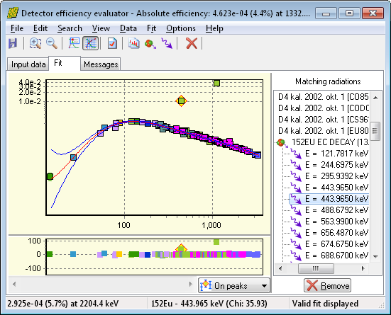
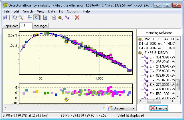
If you check the resulting reduced Chi-squared (RXSQ=101) or the residual of the fit, it is immediately obvious that there is a problem with the fit.

Please be aware of the outlying 152Eu data points on the previous figure, which are far off from the efficiency curve. This is the 443keV line of 152Eu, and it is improper for calibration purposes because the level scheme contains two overlapping 443keV peaks. The similar problem exists with the 1112keV line of 152Eu EC decay and the 1109keV line of 152Eu β- decay.

It is unavoidable to remove all of these disturbing lines. Select the first 443keV line by clicking on it (on the fit chart, or on the residual, or in the list of matching radiations), and then click Remove button, and repeat this for the other problematic line at 443keV. You can use the View/ Sorting of radiations menu to display energy-sorted lines. Also repeat with 1112keV and 1109keV lines of 152Eu, and the notoriously weakly fitted 79keV line of 133Ba.

With those modifications, the RXSQ value goes down to around 3, which should also be improved.

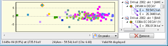
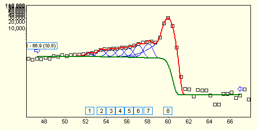
It is better to check the residuals now, to see which line exactly causes this problematic RXSQ:. Click on the outlier point at 59keV. It is immediately displayed on the right that it belongs to 241Am.

In order to see the spectrum's details, save the efficiency fit, and open the 241Am peak evaluation.

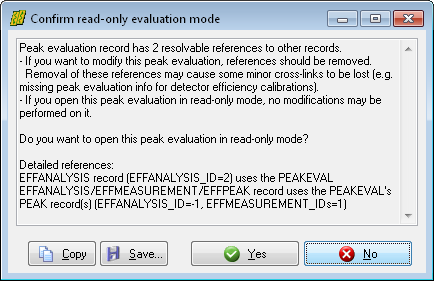
If you have a warning about that this peak evaluation is already used in an analysis, therefore cannot be modified, then select No here.

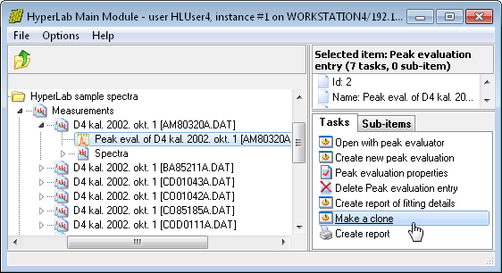
Now select the Make a clone task while the peak evaluation is selected, thus creating a new peak evaluation, which contains the same details as its original one, but editable.

After cloning, a second peak evalution appears on the left, at the database tree.

For the sake of clearer further explanations, we changed its name to 2nd Peak evaluation.

Open this new evaluation, and check the problematic 59keV region.

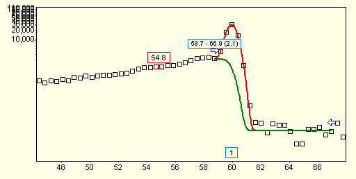
The problem is immediately apparent: the automatic fit incorrectly included part of the background in the peak.

Move the left side of the region to right, by dragging the blue arrow to the base of the peak.

After the manual intervention, the area of the peak decreases significantly (change is over 5%, while its uncertainty was 1%). Now save this peak evaluation.

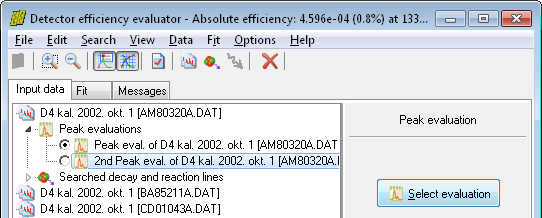
Open the efficiency analysis again.

On the input page, open the 241Am measurement, select on the left the second peak evaluation, then click the Select evaluation button on the right.

After removing two other low-energy lines, the figure shows the improved efficiency curve. It has RXSQ value of 2.7, which indicates a good fit – with only minimum user intervention.

If you have used the cloned peak evaluation, then the original one is possibly unused now, so you can delete it under the measurement entry.