Designating a proper efficiency curve as a default

After a successfully construction of an efficiency curve, you should take one last administrative step: HyperLab should know that this curve is to be used as a default one. This can be done by assigning the efficiency analysis to the measurement setup where it belongs.

After this step, the efficiency of a measurement can be automatically determined, purely by its acquisition date and the measurement setup set up for the spectrum.

This is currently used by HyperLab for two purposes:

nuclide identification is more convenient, as automatic loading of the matching efficiency curve is performed during spectrum deconvolution, and
it is possible to generate an efficiency-corrected peak list (however, this is rarely used).

In order to assign an efficiency analysis to the measurement setup, please follow the instructions below.

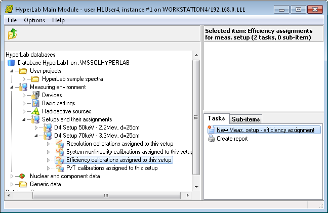
Open Measuring environment node in your database browser tree, then Setups and their assignments, finally the measurement setup where your efficiency curve is created. In our example, the measurement setup 'D4 Setup 70keV – 3.3Mev, d=25cm' was opened. After that entry, click Efficiency calibrations assigned to this setup, and then select the task at the right named New Meas. Setup – efficiency assignment.

A data entry window appears now.

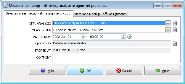
Now you should select the efficiency analysis you have created.

Another important field is the Valid from entry, where you can define the starting date when your efficiency analysis should be used as a default.

Set it to the date of the measurements which have been used for the analysis.

In our example, we set this date to January 1st 2002, to make sure that it will be automatically used for all measurements taken from the very first day of the year.

You should always register a successfully created analysis as default. This way a chain of efficiency curves will be created, each representing a time range of your measurement system, when that calibration was valid.

On this picture we depict a situation when 4 efficiency analysis, Eff1 … Eff4 is assigned to the same measurement setup.

After the first assignment (Eff1), a default efficiency curve is existing in the system.

For example, if a measurement is loaded into peak evaluator, where the acquisition time is between the 2nd and the 3rdefficiency analysis (between Eff2 and Eff3), theEff2 efficiency curve will be automatically loaded, and the isotope identification will use that automatically.